Vanishing Gradients
- 8 minsDisclaimer
This is a discussion on an old problem that hindered the Machine Learning research for decades, now partially solved using various methods discovered in last 10 years. The audience are expected to have basic understanding of Neural Networks and Backpropagation to reap maximum benefit out of the explanations followed.
Neural Networks and Deep Neural Networks
We all are beholding the captivating wizardry of Deep Learning in various applications. With Deep Learning, tedious tasks of past like Translation, Image Recognition, Object Detection and Speech Recognition are now working par with human level accuracy. There must be some spell, Deep Learning is casting, to perform these sophisticated tasks, isn't it? :D
Let's answer that question first, shall we? So, what is "Deep" in Deep Learning?
Obviously, it is the depth of the architecture or simply put, it is the number of layers we add to a shallow network to make it deep.
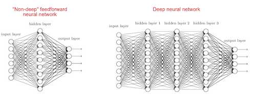
The next question is why more layers?
As the number of layers increases, deep networks can represent very complex functions. It can also learn features at many different levels of abstraction, from edges (at the lower layers) to very complex features (at the deeper layers). Consider an image recognition example below. As we all know, in image recognition, Deep Networks surpassed human level accuracy.
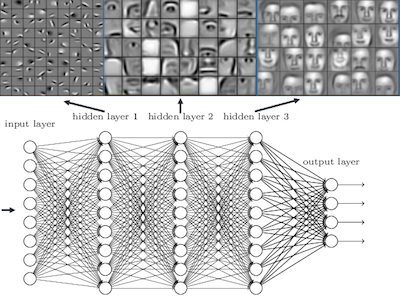
As we see, the initial layers can detect the naive patterns like edges, then middle layers learn more complex patterns like nose, lips etc. and finally, the deepest layers learn the entire face. Woo-Hoo!!
So the point is, **depth matters** and it is helpful to learn more and more details from the input. Next time when we confront a complex problem to be solved by Deep Learning, what would be the first fix, if patterns are not learned well? Leo knows the solution :D

What is wrong with Deep Neural Networks ?
Everything in this world has it's price. Though, the power of deep networks is immense, training a deep network is not that easy. No, I'm not talking about the hardware limitations which is indeed a practical problem. But in litrature, there are many fundamental issues we face while training deep networks.
Now, you may get deluded a bit, thinking that these issues are due to complex architectures of deep networks. In contrast, root of these issues are linked with learning algorithms like backpropagation, we use to train them.
Wait, what? Reputation of backpropagation is on the line? :o
Yeah, kind of :D
Let’s make a brief discussion on what actually happens in backpropagation. For that, consider the following network.
It is not deep enough :/
But helpful for explaining the concept :P

For simplicity, we are going to make some assumptions.
- Biases are zero
- Activation function $g$ is identity function in all layers.
- So, effectively, it is as good as it gets, there is no activation.
- Please not this point carefully since, it is going to make a lot of easiness in our calculations.
These assumptions are odd :/
We’ll come back to a fully fledged example once we answer the question stated in section heading :)
Okay :/
We compute a cost $J$ on forward direction, traversing from first layer to last layer. This is called feed forward propagation. This cost function tell us about the error between the expected output $y$ and computed output $\hat y$.
How do we calculate $\hat y$ ? It is the product of activations of each layer.
Layer 1 output, $Z^1$ = $W^1 * X$
Activation of layer 1, $A^1$ = $g(Z^1) = W^1 * X$
Layer 2 output, $Z^2$ = $W^2\ *\ Activation\ of\ layer\ 1 =\ W^2 * W^1 * X $
Activation of layer 2, $A^2$ = $g(Z^2) = g(W^2 * W^1 * X) =\ W^2 * W^1 * X$
Layer 3 output,
\[Z^3\ =\ W^3\ *\ Activation\ of\ layer\ 2 =\ W^3 * W^2 * W^1 * X\]Activation of layer 3,
\[\hat y\ or\ A^3\ =\ g(Z^3)\ =\ g(W^3 * W^2 * W^1 * X ) = W^3 * W^2 * W^1 * X\]Then,
\[\hat y\ =\ W^3 * W^2 * W^1 * X\]Cost or Error, $J$ = $\hat y\ -\ y$ = $A^3\ -\ y$
To perform this minimization process, Gradient Descent is going to adjust the parameters, i.e. weights of our network. This is the so called "learning" part in Deep Learning.
First, it'll calculate gradients/derivatives of cost function with respect to parameters of final layer. But, that gradient depends on previous layer parameters since the layers are stacked one on another. So we need to calculate previous layer gradients, and substitute those values in current layer equations. The entire network follows this pattern.
I know you’re scratching your head :D Let’s represent it mathematically.
Since the activation is identiy, $\frac{\partial A}{\partial Z}$ will be always 1. We'll substitute this condition in following equations.
For second layer,
\[\frac{\partial J}{\partial W^2}\ = \ \frac{\partial J}{\partial A^3} * \frac{\partial A^3}{\partial Z^3} * \frac{\partial Z^3}{\partial A^2} * \frac{\partial A^2}{\partial Z^2} * \frac{\partial Z^2}{\partial W^2}\] \[\frac{\partial J}{\partial W^2}\ =\ \frac{\partial (A^3\ -\ y)}{\partial A^3} * 1 * \frac{\partial (W^3 * W^2 * W^1 * X)}{\partial (W^2 * W^1 * X)} * 1 * \frac{\partial (W^2 * W^1 * X)}{\partial W^2}\\\\\] \[\frac{\partial J}{\partial W^2}\ = 1 * W^3 * W^1 * X\]And finally,
\[\frac{\partial J}{\partial W^1}\ = \ \frac{\partial J}{\partial A^3} * \frac{\partial A^3}{\partial Z^3} * \frac{\partial Z^3}{\partial A^2} * \frac{\partial A^2}{\partial Z^2} * \frac{\partial Z^2}{\partial A^1} * \frac{\partial A^1}{\partial Z^1} * \frac{\partial Z^1}{\partial W^1}\] \[\frac{\partial J}{\partial W^1}\ =\ \frac{\partial (A^3\ -\ y)}{\partial a^3} * 1 * \frac{\partial (W^3 * W^2 * W^1 * X)}{\partial (W^2 * W^1 * X)} * 1 * \frac{\partial (W^2 * W^1 * X)}{\partial (W^1 * X)} * 1 * \frac{\partial (W^1 * X)}{\partial W^1}\\\\\] \[\frac{\partial J}{\partial W^1}\ = 1 * W^3 * W^2 * X\]We call this circus, Chain rule in calculus :D So a computational train starting from final layer, "propagates" upto first layer and thus the name "Back Propagation" :P
Now, what is essentially "back propagated"? It's the gradients which represents the rate at which the error changes with respect to parameters in each layer!
If everything goes right, i.e. all gradients are calculated finitely, then we'll be able to update every weights and biases in the network at the end of one epoch. Intuitively, the updation of parameters reflects how the change in network output is going to affect the parameters in various layers. This process is cycled until a certain number of epochs or definite admissable error is reached. Now we're ready to understand the problem of vanishing gradients in detail.
Let’s imagine, if all weights are same $W$, we can consider two possible cases for the value $W$.
You are making a lot of assumptions. And this one is ridiculous. Rule number 1 is you shall not use same weights in a neural network :@
I know :)
That symmetry will result in useless linear learners :@
I know that too, are you done? :)
NO ! Yeah … yes :@
This assumption is solely intended for getting a better understanding of the issue. Let’s continue :)
Here we have 3 layers, but let’s generalize for $L$ layers.
a. $W>I$ for I = Identity matrix
\[\frac{\partial J}{\partial W^1} = W^L * X\]Since W is greater than 1, the resulting value will be exponentially high. This is called Exploding gradients.
b. $W<I$ for I = Identity matrix
\[\frac{\partial J}{\partial W^1} = W^L * X\]Since W is less than 1, the resulting value will be exponentially decaying. This is called Vanishing gradients.
The victims
Let me ask you something, How severe vanishing gradient is going to each layer? ;)
Gradients are everywhere, so it should be the same effect, right?
So, the middle layer and first layer are affected equally? ;)
Explain :/
No, it’s not. Why? Let’s consider the same network with sigmoid activation and weights are not same anymore :D
We know that sigmoid function, \(S\ =\ \frac{1}{1+e^-x}\)
Derivative of sigmoid function, \(\frac{\partial S}{\partial x}\ =\ \frac{e^-x}{(1 + e^-x)^2}\)
Now, let’s calculate the gradients in final layer and first layer.
\[\frac{\partial J}{\partial W^3}\ = \ \frac{\partial J}{\partial A^3} * \frac{\partial A^3}{\partial Z^3} * \frac{\partial Z^3}{\partial W^3}\] \[\frac{\partial J}{\partial W^3}\ =\ \frac{\partial}{\partial A^3}(A^3\ -\ y) * \frac{e^{-Z^2}}{(1 + e^{-Z^2})^2} * \frac{\partial}{\partial W^3} (W^3 * W^2 * W^1 * X)\] \[\frac{\partial J}{\partial W^3}\ = 1 * W^2 * \frac{e^{-Z^2}}{(1 + e^{-Z^2})^2} * W^1 * X\]
\[\frac{\partial J}{\partial W^1}\ = \ \frac{\partial J}{\partial A^3} * \frac{\partial A^3}{\partial Z^3} * \frac{\partial Z^3}{\partial A^2} * \frac{\partial A^2}{\partial Z^2} * \frac{\partial Z^2}{\partial A^1} * \frac{\partial A^1}{\partial Z^1} * \frac{\partial Z^1}{\partial W^1}\] \[\frac{\partial J}{\partial W^1}\ = 1 * \frac{e^{-Z^3}}{(1 + e^{-Z^3})^2} * W^3 * \frac{e^{-Z^2}}{(1 + e^{-Z^2})^2} * W^2 * \frac{e^{-Z^1}}{(1 + e^{-Z^1})^2} * X\]
As we see, gradient at final layer goes through only 3 multiplications and first layer requires seven. Consider the following calculation and you'll understand what I'm getting at.
\[0.99^3 = 0.970299\] \[0.99^7 = 0.9320653479\] \[0.99^{100} = 0.36603234127\] \[0.99^{300} = 0.04904089407\]As we propagate away from final layer, the perturbation on network output will not reach the layers, even if reaches, the gradient will be too feeble to make an update. This issue get worsened when number of layers increases. Very deep networks often have a gradient signal that goes to zero quickly because of this reason, thus making gradient descent unbearably slow. More specifically, during gradient descent, as we backprop from the final layer back to the first layer, we are multiplying by the weight matrix on each step, and thus the gradient can decrease exponentially quickly to zero. Gradient based methods learn a parameter's value by understanding how a small change in the parameter's value will affect the network's output. If a change in the parameter's value causes very small change in the network's output - the network just can't learn the parameter effectively.
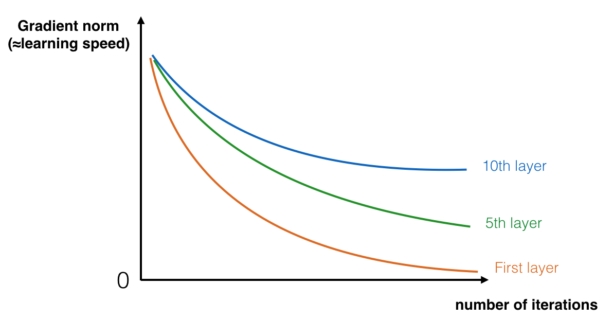
The speed of learning decreases very rapidly for the early layers as the network trains
So, which layer is going to suffer the most? Obviously the initial layers. Now think about it, in image recognition we saw that initial layers are the learning the building blocks like edges, if they are learned wrong, then you know...
So that’s it. We defined the problem pretty comphrehensive. Now do we have any remedies?
Remedies
Well I've a sad news for you. There is no complete cure for vanishing gradient yet, but we've some remarkable advancements to reduce the effect. We'll discuss some techniques and it's consequences.
Initializing the weights with standard techniques like Xavier Intialization
Initializing weights properly can reduce to some extend since the fact both too high or too low weights can result in exploding/vanishing gradients.
The curse of Sigmoids and Tanhs
We saw Sigmoid function above used as the activation in our network. Let’s see the graph of this function and it’s derivative.
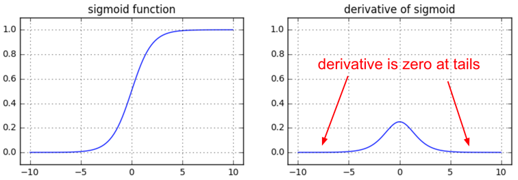
Let’s make some observations from these graphs.
a. Sigmoid is confined to the interval $[0,\ 1]$, the output will be always between these interval for any input.
Even if we consider to initialize the weights as big as say $[-400,\ 400]$, after the activation, that will a binay matrix. High values tend to 1 and low values to 0. This will make derivatives zero and thus vanishing gradients.
b. The maximum value of derivative of sigmoid function is 0.25
So by default, the input weights get $(\frac{1}{4})^{th}$ of the original value on calculating the gradients, since derivative $\frac{\partial A}{\partial Z}$ is multiplied with it.
Same are applicable to tanh which is an extended sigmoid.
So the take away is don’t use them :D
Dying ReLUs
Let’s plot Rectified Linear Units and it’s derivative.
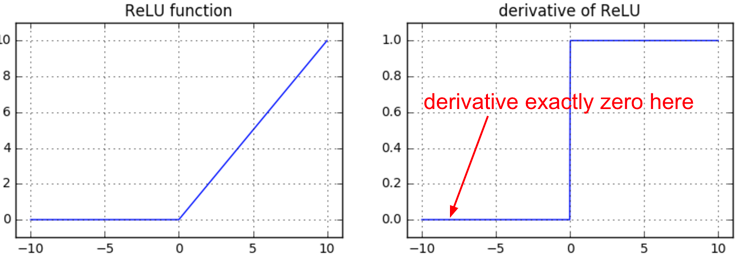
What are the observations?
a. ReLUs don’t suffer from limited interval problem like sigmoid. The minimum value is 0 but there is no limit for maximum value.
b. If the input value is less than zero, then output and derivative are zero.
This will eliminate all the negative inputs which is okay. But derivatives getting zero is a problem. This means, in the entire training, that neuron which can't fire above zero will remain unlearned or dead.
So, ReLU is also not the perfect solution, but provides a great relief.
Gating mechanisms in Long Short Term Memory Cells (LSTMs) and Gated Recurrent Units (GRUs)
In sequence learning, the issue of exploding/vanishing gradients is dire, the gated architecture helps to reduce the effect. Read about this in real detail at here.
ResNets
Deep Residual Learning for Image Recognition by Kaiming He, Xiangyu Zhang, Shaoqing Ren and Jian Sun at Microsoft Research provides a new architecture to solve the problem of training deep networks.
Now let me tell you the story behind this whole tutorial on Vanishing Gradients. I wanted to write a tutorial on ResNets paper, but when started I had this feeling that without giving a proper definition on the problem we are going to solve with ResNets, the whole tutorial would be incomplete. So I started working on this tutorial, which you may find as a preamble to ResNets tutorial :D So that's it. See you in ResNets tutorial.
Cheers :)

Sleeba Paul
Dreamer | Learner | Storyteller