Language Modelling using Recurrent Neural Networks (Part-2)

Sunday. August 12, 2018 - 14 mins

Disclaimer

The audience is expected to have the basic understanding of Neural Networks, Backpropagation, Vanishing Gradients, and ConvNets. Familiarization of PyTorch is appreciated too, as the programming session will be on it.

Introduction

In the previous post, we briefly discussed why CNN’s are not capable of extracting sequence relationships. The fundamental reason for that failure is the assumption of independence between the training examples. Say, in an image classification problem, each image is a data point and each image is considered as an independent example.

But use cases like processing frames from video, snippets of audio, and language, the assumption of independent examples fail. Here, data points related in time and thus they are named as sequence problems. We need a new architecture which can capture the temporal relationship in sequence problems.

In this post with let’s unfold Language modeling, a well-defined sequence problem and then dive deep into RNNs which can solve it.

Language Modelling

In simple words, language modeling is generating the next token (it can be a character or a word) in accordance with previous tokens (again words or characters).

In the previous post, we’ve seen many examples of it.

1. Sleeba is native of Kerala. He can fluently speak _____.
2. I bought my poodle from Paris. He barks _____.
3. I bought my poodle from Paris when I was staying with Sleeba. He has this trait of nodding while having food. But he loves __.

Here as you see, the past context is really important to predict the next token. If we miss that, then the entire sequence/sentence becomes meaningless. So the problem is defined. How to represent it in mathematical terms?

Don’t panic. We can explain that 😁

It is as simple as,

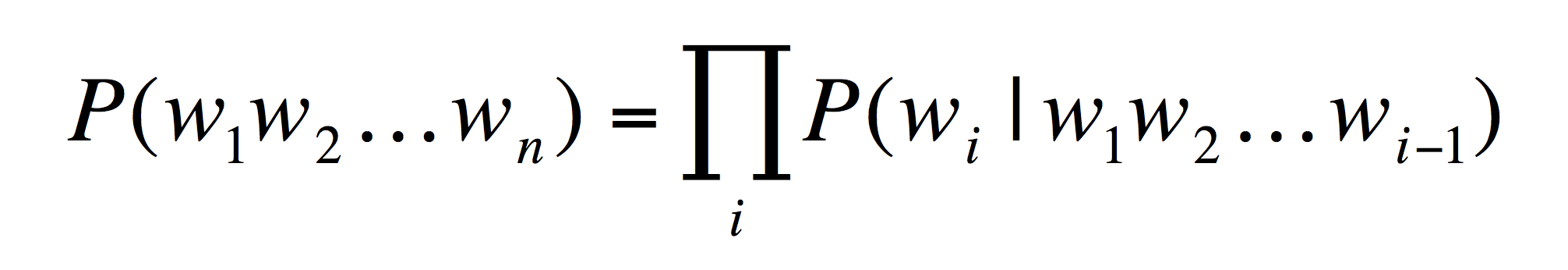
P(Is Trump linked with Stormy Daniels?) =
P(Is) x
P(Trump | Is) x
P(linked | Is, Trump ) x
P(with | Is, Trump, linked) x
P(Stormy | Is, Trump, linked, with) x
P (Daniels | Is, Trump, linked, with, Stormy) x
P (? | Is, Trump, linked, with, Stormy, Daniels)

As we can see, the probability of each word is conditioned on previous words, thus the context is well maintained throughout the sentence. So if we can learn these past probability distributions, then we can generate the next word accordingly.

This has become so weird. That equation takes after an iguana 😑

Really? 😆

Conditional probabilities, a lot of mathematical mess… But these tasks are as easy as pie for us 😐

That’s the thing about homo sapiens. We are cool in many ways 😎

We can do language modeling in two levels

• Character level which generates a character at a time.

• Word level which generates a word at a time.

Dictionary

A language model will always have a dictionary, which is a collection of all the tokens that will be used in that model. For example, the dictionary of a character language model of English will be the collection of 26 small letters, 26 capital letters, space and special characters of English. Dictionary size is small, still, we can generate the entire English vocabulary.

What about word level representation? Dictionary will contain all the words present in our training data. We can’t expect the model to generate a new word which is not in the vocabulary. Same time, word level model is less gibberish than a character model since a word is the basic meaningful building block of a sentence.

Simplest language model

The simplest language modeling is randomly picking each character from its dictionary. The below code snippet depicts the simple character level language model. You may try a word level language model by yourself.

Generated Sentence is,

W>X^Spz,wGOr(!C?uac-DqXvX_b^lv/S^p~cs)NjKWz;O+j"cZn jwZRK=I(xdD>tjgjF[BTc.mii`l<b/x#/,}(lIn\t":Ij&im

Though this approach is simple to implement, we fail to maintain the context. The probability of every character generated is the same ($\frac{1}{Dictionary\ size}$). It is not conditioned on previous inputs. Thus the generated text is gibberish.

Can we do better?

Recurrent Neural Networks (RNNs)

RNNs are entirely different from usual neural networks when it comes to architecture. If CNNs are best for spatially distributed data, RNNs are specially designed for processing sequential data. They are not a new topic in the Deep Learning history either. In 1982, John Hopfield published a paper in the context of cognitive science and computational neuroscience which contained the idea of RNNs. From that paper to Google Duplex, which can take an appointment for us by building a reliable conversation with a barber, we’ve traversed a lot in this domain.

Let’s jump into the notations in order to understand the architecture of RNNs.

Notations

Imagine $x$ is the input sentence/sequence goes a black box named RNN and we get an output word $y$ for our language modeling problem.

Using temporal terminology, an input sequence consists of data points $x^t$ that arrive in a discrete sequence of time steps indexed by $t$.

I don’t know why plain English is not a criterion, when it comes to describing something scientific or mathematical 😖

Let me help you 🤣

Actually, this is a simple concept. For example, in the word level language modeling, sequence

I support LGBT rights

$x^1$ = $I$, $x^2$ = $support$ and so on.

While in character level,

$x^1$ = $I$, $x^2$ = $'\ '$, $x^3$ = $s$, $x^4$ = $u$ etc.

If you’ve noticed, we don’t need space token for word-level modeling since words are obviously separated by space.

Next question is, how to represent this word/character mathematically? There are many ways to do that and it is worth another blog post. Here we will briefly discuss two types.

One hot vectors (Sparse representation)

Imagine your dictionary is [rights, human, LGBT, equality, I, support, a]. Vocabulary size is 7. Now, let $x$ be the input sentence I support LGBT rights, then representing support in the sentence will be,

$x^2\ =\ \begin{bmatrix}0 & 0 & 0 & 0 & 0 & 1 & 0\end{bmatrix}$

What if the vocabulary size is $100000$. Then $x^2$ will be a $(1$ x $100000)$ matrix with a $1$ and a hell lot of zeroes. That’s why it is sparse representation. As the dictionary size increases, the computational and memory cost of one-hot representation increases. But most importantly, it skips the relationship between words, which is less intuitive. Read more about one-hot encoding at here.

Word embeddings (Dense representation)

Word embeddings cover up all the pitfalls of one hot vectors. They are learned using unsupervised methods like autoencoders.

Firstly, their representation vector size don’t increment with the vocabulary size. For almost all the embedding algorithms, the vector dimensions are fixed.

For example, GloVe: Global Vectors for Word Representation by Jeffrey Pennington, Richard Socher and Christopher D. Manning from Stanford, converts the word “LGBT” to a 300 dimension vector. In a 300 dimension space, LGBT vector will be close to the 300 dimension vector of human to represent the relationship that the LGBT community is also the part of homo sapiens.

At the end of the day, for example, the sample dense vector of LGBT will be,

$x^3$=$\begin{bmatrix}0.2218 & 0.3812 & 0.8845 & …\end{bmatrix}$

Secondly, they are not just ones and zeros but decimals representing the relationship a word between other words. Thus they are dense representations. Using these word embeddings, interesting relationships that can be learned like King - Man + Woman = Queen, India to New Delhi is Thailand to Jakarta etc.

I’m not going to explain how these decimals are generated. But from the above explanation, if you get the gut feeling that the black box RNN will be able to map the context more intuitively with word embeddings than one hot vectors, then that’s enough for this tutorial 😁 But I highly recommend to read about embeddings at here, here, here, and here since wisdom is sexy.

Architecture

Usually, when you search for an RNN tutorial, you get the image given below. This is largely inspired by Christopher Olah’s famous blog post on Understanding LSTM Networks.

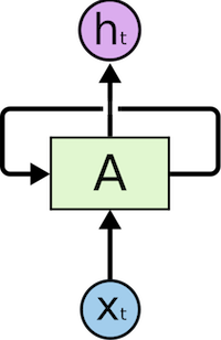
A single RNN unit recursed to itself. But, this representation has two rudimentary confusions.

• It is a cyclic graph representation

All the feed forward neural network graphs we’ve seen yet are acylic. CNNs structures we’ve seen are acyclic. Particularly, they are directed acyclic graphs (DAG). They start from the input nodes and reach the output nodes without loops.

Why this is important?

The mighty back propagation is defined only for acyclic graphs. So we can’t apply our learning algorithm in this RNN representation. Thus we move to the unrolled architecture.

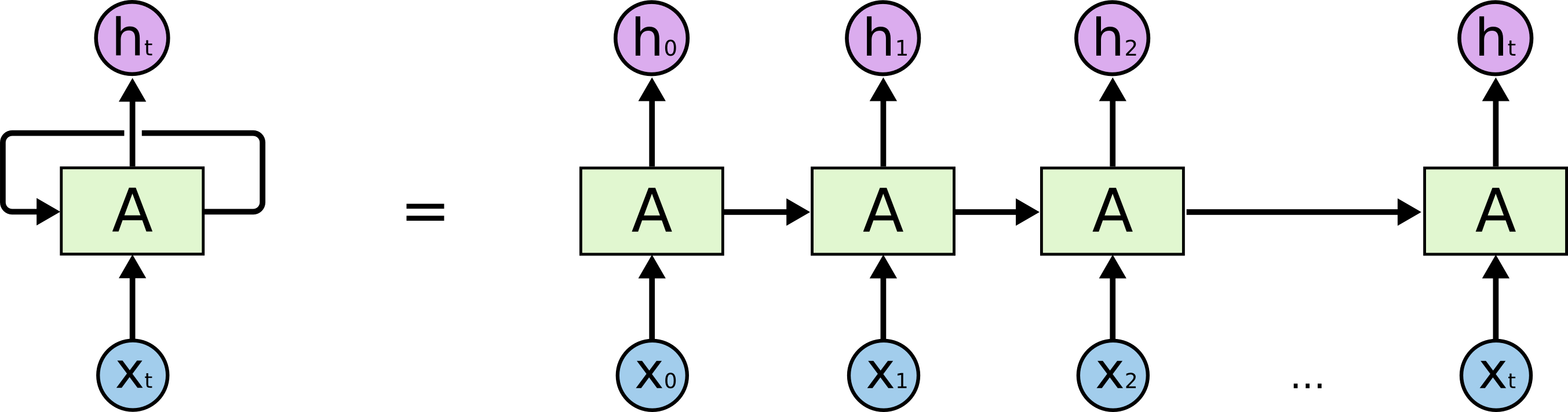
Or more intuitively,

Here the single cell recursed to itself is unrolled to a sequence of cells. This is an acyclic architecture. Now backpropagation is possible and it has a fancy name too. Back Propagation Through Time (BPTT).

But there is the second issue.

• We’ve learned all the neural network architectures in neuron level, but this is a cell level explanation.

In this post, I’m planning a neuron level explanation of an RNN cell. To start with, let’s define the equations of an RNN cell.

Equations

Let’s begin with $h^{[t-1]}$, the hidden state input from previous RNN cell to current cell (Refer the diagram above).

• $h^{[t]}\ =\ F(W_{hh} \cdot h^{[t-1]}\ +\ W_{xh} \cdot x^{[t]} + b_h)$

A hidden state? 🤷 Why we need a state now? We never had a state vector for CNNs. Why now?

Remember we talked about maintaining context of a sentence? For this purpose, we need the information from past. $h^{[t-1]}$ is our guy who carries the baton of past. I love to call $h^{[t-1]}$ the context vector rather than a hidden state vector since it carries the past context of the sequence.

Now let me show you the beauty of RNN architecture with this equation.

We feed context vector ($h^{[t-1]}$) from past and the current input $x^{[t]}$ to an RNN cell to get the future ($h^{[t]}$) of the sequence.

Perfect, ain’t it? 💯

Now have a closer look at the equation. We’ve two weights, $W_{hh}$ and $W_{xh}$ which are going to adjusted or learned while we train these cells with examples. What are these weights going to learn?

$W_{hh}$ will learn what needs to remember or forget from past $h^{[t-1]}$. $W_{xh}$ learns about contribution of current input $x^{[t]}$. Together with both $W_{hh}$ and $W_{xh}$ we will build our new context vector $h^{[t]}$ which has information from past and present. We’re going to use this new context vector for two things.

Let’s go to the next equation for the first application.

• $y^{[t]}\ =\ W_{hy} \cdot h^{[t]}\ +\ b_y$

We’re generating an immediate output $y^{[t]}$ using the current context $h^{[t]}$ where $W_{hy}$ learns about creating an output from current context. Note that, this is a completely optional decision and depends on the application. The model we are discussing now is (Many to Many Synced) rightmost model, ideal for language modeling.

Have a look at the figure given below which depicts different architecture using RNNs for sentiment analysis, machine translation, photo description etc.

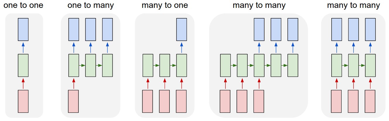
(This picture, as well as many key ideas, are taken from the bible of blog posts on RNNs, The Unreasonable Effectiveness of Recurrent Neural Networks by Andrej Karpathy ❤️)

One more thing which is important to be mentioned is the RNN network architecture for language modeling. Here, prediction of previous cell $y^{[t-1]}$ is passed as the input $x^{[t]}$ to next cell. Have a brief look at these variables in the above figure. Why such an implementation?

It is simply because we are dealing with a continuous stream of text. The previous word is our lucidly our current input.

Again, this is not the universal network architecture. There are variations like teacher forcing, which don’t follow this pattern. On that note, let’s move to the third equation.

• $o^{[t]}\ =\ softmax(y^{[t]})$

The third equation is not really a part of the architecture. The softmax layer will convert the output of RNN into a probability distribution. In language modeling, it will be a distribution with a population of dictionary size. An ideal network will predict the maximum probability for that word or character which is most likely to come next, considering the past context.

The second application of the context vector is to pass the baton to the next time step.

Wait, what is F?

Oh! I forgot about that. F is our good old non-linear activation function from feedforward networks. Like tanh, ReLU etc.

You’re careless 😏

Oh! Come on 🙄

Neuron Level representation

We’ve seen the insanely intuitive equations on an RNN cell. But let me unveil these cells at a neuron level so that you may understand it thoroughly.

Let’s go back to equation 1. Consider non-linearity $F$ as tanh.

• $h^{[t]}\ =\ tanh(W_{hh} \cdot h^{[t-1]}\ +\ W_{xh} \cdot x^{[t]} + b_h)$

Let’s break this equation down,

What is $W_{hh} \cdot h^{[t-1]}$ ? It’s a linear transformation or a simple neural network layer we’ve seen in many normal neural networks.

What about $W_{xh} \cdot x^{[t]}$? Another linear layer.

Now, you must have got the idea of the second equation too. Let me unveil the neuron level RNN cell to you. Brace yourself, ladies and gentlemen… Pooooffff !!! 🌟✨✨⚡

Current input and past context vector are linearly transformed and summed together. This sum is then passed to a $tanh$ to inject non-linearity/activation. Thus current context vector is generated, which is used for generating an optional output and pass the context to the next time step. (I didn’t add a bias member explicitly, but you got the idea anyway 😊)

I think this my diagram is pretty self-explanatory.

But it is little big. Christopher Olah chose the simpler diagram for a reason 🤔

Agreed. I’ll confine it to the following.

AAAAAAAGHHH 🤩🤩🤩 Finally I explained RNN in neuron level. I’m feeling good. Really really good. I can die in peace now.

Okay, die well 😜

Nope… Actually, I was overreacting… a bit 😬

A bit?

😀

Note

People always have confusion when the hyperparameter hidden size and sequence length of RNNs are discussed. Now from the neuron level diagram, we can clearly understand that hidden size is the number of neurons present in the hidden layer. Here it is three.

output size can be sometimes referred as the hidden size as RNN has two outputs i.e. $y$ and $h^{[t]}$. As $y$ is optional, sometimes we treat $h$ as output.

For good models, provided we’ve enough data(say, 100 million characters) we can afford to use a large hidden size. For small data samples (< 10 million characters) use small hidden size values.

sequence length is the number of RNN cells unrolled/considered at once or simply it is the number of time steps.

Now we’ll discuss two most important concepts of RNNs and wrap up the talk and jump to code since,

Talk is cheap. Show me the code - Linus Torvalds

Parameter Sharing

Let’s talk about the parameter sharing of Neural Networks in general and understand the parameter sharing of RNN in a comparative level.

There is no parameter sharing in normal feed-forward networks. Every layer has a bunch of individual weights and biases and there are learned/updated on backpropagation.

But when it comes to CNNs, we dramatically reduce the number of parameters using filters. The number of parameters is defined from size and depth of the filter. Combination of these parameters is used for representing all the patterns. Thus we can say that these parameters are reused or say shared to represent different patterns. Sharing helps to reduce the numbers parameters. The same idea is used in RNNs too but in a slightly different way.

CNNs share parameters for representing spatial features. RNNs does it through time for imbibing temporal features. This is implemented by updating the same weights on every time steps.

What does that mean? 🤔

Let me explain the training of RNNs 😊

Training of RNNs

First of all, the number of cells and number of timesteps are the same. Don’t confuse them layers. Multiple layer RNNs look something like this.

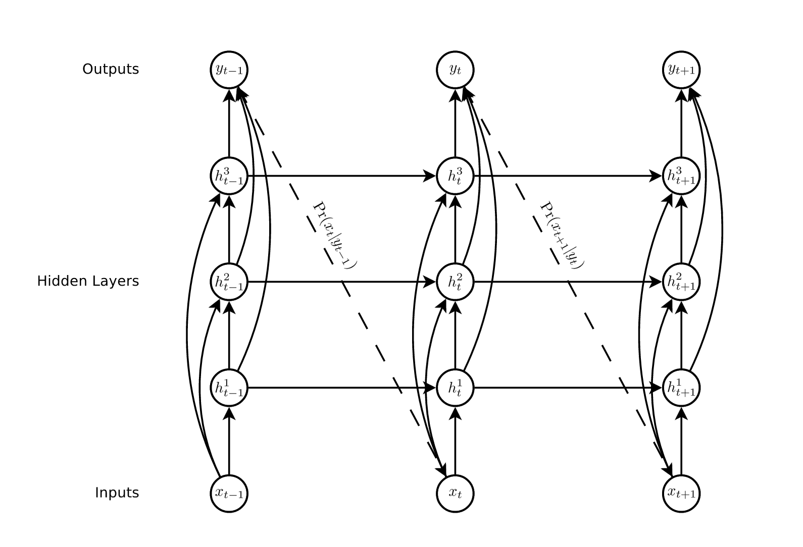
Now, for example in a layer, we’ve 3 unrolled RNN cells, i.e 3-time steps.

In the first cell, we feed our context vector $h^0$ and current input word $x^0$. Initial context vector $h^0$ is will be a zero vector as we don’t have any context from the past yet. Though we’ve three cells unrolled, all of them don’t have individual weights. Instead, they share the same weights $W_{hh}$, $W_{hx}$ and $W_{hy}$.

Okay. So there are three cells but there are only a single set of weights 🤔

Yes. That’s right.

But how it is implemented?

In this particular case of language modeling, we need to predict the next word/character at each time step as shown in the figure. That means, we need to update the weights at each cell. Implementing the idea of parameter sharing here means we update the same weights at every cell during backpropagation. Here, during a backpropagation, there will be three updates to weights. (Though this is the theory, in practice, we don’t update weights after each step to maintain stability. Usually, the loss of each step are added and at the end of the sequence we backpropagate once with respect to accumulated weights.)

Okay, we understood the idea of parameter sharing. Why is it important? Yes, indeed it will reduce the parameters, but more than that, there is another bonus for a sequence problem.

Imagine the following sentences.

1. Kids are lovely.
2. Kids of Jessie are lovely.

Here, kids is plural and should be followed by a plural verb like were. Note that, the position of kids or were doesn’t matter for such a relationship. If we train a feed-forward network for learning this relationship, we would need parameters to be learned at every position of the input sentence. In that case, every relationship should be learned at every position. It is not practical. While we share parameters across the parts of the sentence, it becomes position and length agnostic, therby generalizes the relationships well.

Backpropagation Through Time (BPTT)

Training RNNs is not a piece of cake. The villain is the very concept of using RNNs. The dependency of current output on past inputs. To elaborate on this issue, first, we define the loss of our problem.

As I mentioned above, we predict at each every cell. This prediction is compared with the original label. A loss is created here. Usual stuff, isn’t it? But this story is for a time step. What if we’ve such t steps? Let’s take 3-time steps as above.

$Loss,\ L\ =\ L_{1}\ +\ L_{2}\ +\ L_{3}$

The worry begins here. In RNNs, since the parameters are shared, if we need to find a gradient at a time step, then we need to sum up all the gradients from all past time steps.

Let’s bring back equations of RNN cells. For simplicity I’m naming $W_{hh}$ as $W$, $W_{xh}$ as $V$ and $W_{xy}$ as $U$.

• $h^{[t]}\ =\ F(W \cdot h^{[t-1]}\ +\ V \cdot x^{[t]} + b_h)$

• $y^{[t]}\ =\ U \cdot h^{[t]}\ +\ b_y$

Here we need to calculate six gradients of loss with respect to learnable parameters. They are,

$\frac{\partial L}{\partial U}$, $\frac{\partial L}{\partial V}$, $\frac{\partial L}{\partial W}$, $\frac{\partial L}{\partial b_x}$ and $\frac{\partial L}{\partial b_h}$.

Consider the $\frac{\partial L}{\partial U}$ first. Let the number of time steps be $T$.

$\frac{\partial L}{\partial U}\ = \sum_{t=1}^{T} \frac{\partial L_t}{\partial U}$

By chain rule,

$\frac{\partial L_t}{\partial U}\ =\ \frac{\partial L_t}{\partial y^{[t]}}\ *\ \frac{\partial y^{[t]}}{\partial U}$

$\frac{\partial y^{[t]}}{\partial U}$ can be easily found out using our second equation. We’re good since there is only one dependency for $U$ in it. This is for a single layer. You may need to traverse through layers if multiple layers are involved 😊

Now, let’s calculate $\frac{\partial L}{\partial W}$.

$\frac{\partial L}{\partial W}\ =\ \sum_{t=1}^{T} \frac{\partial L_t}{\partial W}$

Using chain rule,

$\frac{\partial L_t}{\partial W}\ =\ \frac{\partial L_t}{\partial y^{[t]}}\ *\ \frac{\partial y^{[t]}}{\partial h^{[t]}}\ *\ \frac{\partial h^{[t]}}{\partial W}$

Easy? Nope. This interpretation is wrong. Because not just $h^{[t]}$, but the whole $h^{[t]}$, $h^{[t-1]}$, … $h^{[0]}$ depends on $W$. So gradients can’t be calculated using just chain rule, we need to go for a total derivative. A big thanks to parameter sharing 😏

So what is the right equation?

$\frac{\partial L_t}{\partial W}\ =\ \frac{\partial L_t}{\partial y^{[t]}}\ *\ \frac{\partial y^{[t]}}{\partial h^{[t]}}\ *\ \sum_{k=0}^{t}\Bigg(\prod_{i=k+1}^{t} \frac{\partial h^{[i]}}{\partial h^{[i-1]}}\Bigg)\ *\ \frac{\partial h^{[k]}}{\partial W}$

Same goes for bias $b_h$

$\frac{\partial L_t}{\partial b_h}\ =\ \frac{\partial L_t}{\partial y^{[t]}}\ *\ \frac{\partial y^{[t]}}{\partial h^{[t]}}\ *\ \sum_{k=0}^{t}\Bigg(\prod_{i=k+1}^{t} \frac{\partial h^{[i]}}{\partial h^{[i-1]}}\Bigg)\ *\ \frac{\partial h^{[k]}}{\partial b_h}$

$\frac{\partial L}{\partial V}$ and $\frac{\partial L}{\partial b_x}$ will be having similar equations.

That’s the meanest thing I’ve seen in 2018 🤦‍

😂

Yes, these equations seem complex. But we can interpret them really well to get the intuition.

• Normally, for training a neural network, we need to backpropagate through just layers. To train RNN, we need to backpropagate through not just layers but time steps as well.

• What exactly the above equation tells us? It is depicting the contribution of a state of the network in the past time step $k$ to the gradient of the loss at the current time step $t$. Yes, blame to parameter sharing.

• The more the time steps between $k$ and $t$, the more elements in this equation.

Vanishing and Exploding Gradient Problem

Can you see a factor $\frac{\partial h^{[i]}}{\partial h^{[i-1]}}$ in the above equation. It is a Jacobian matrix. Let’s consider two cases of the norm value of this matrix.

• $|\frac{\partial h^{[i]}}{\partial h^{[i-1]}}|\ >\ 1$

The product goes exponentially fast. This makes learning unstable. The gradient can shoot up to $NaN$. This is exploding gradients.

• $|\frac{\partial h^{[i]}}{\partial h^{[i-1]}}|\ <\ 1$

The product goes to $0$ exponentially fast. Thus long-term dependencies from past won’t be reflecting on current output. Contributions from far away steps will vanish. This is called vanishing gradients.

These two are the most challenging issues we face when we try to train the RNNs. There are mitigation strategies for both these issues. I’ve written a decent detailed post on them and you may read it here.

So that’s it. I know it was a long journey. But this is worth the effort considering the cool applications around us. Now let’s see all these blah blah blahs in action. I’ve shared a Google Colab notebook in the following link.

Programming session link: https://drive.google.com/file/d/12pEy-aOS0_PiVkFgxyINmBbtuvB5TqV5/view?usp=sharing

Sleeba Paul

Dreamer | Learner | Storyteller

Tweet Share

comments powered by Disqus