
Residual Networks
- 7 minsDisclaimer
This is a tutorial on the paper Deep Residual Learning for Image Recognition by Kaiming He, Xiangyu Zhang, Shaoqing Ren and Jian Sun at Microsoft Research. The audience is expected to have basic understanding of Neural Networks, Backpropagation, Vanishing Gradients and ConvNets. Familiarization of Keras is appreciated too, as the programming session will be on it.
This tutorial will focus mostly on the ResNet paper contents. If the reader would like to have a preamble, I’ve written a comphrehensive discussion on issues which are addressed by ResNets at here. If you’re a beginner, this discussion is highly recommended.
Using ResNets, in the ImageNet challenge 2015, the Microsoft team won first place in all three categories it entered: classification, localization and detection. Its system was better than the other entrants by a large margin. In the Microsoft Common Objects in Context challenge, also known as MS COCO, the Microsoft team won first place for image detection and segmentation.
Let’s learn together the magic of Resnets, shall we? :)
What is wrong with Deep Neural Networks ?
ResNets paper starts with asking this question. Deep Neural Networks can learn the most difficult tasks, but training them was always been an obstacle in Deep Learning research. There are mainly two issues researchers confront,
- Vanishing Gradients
Vanishing Gradient Problem is a difficulty found in training Artificial Neural Networks with gradient based methods (e.g Back Propagation). In particular, this problem makes it really hard to learn and tune the parameters of the earlier layers in the network as the gradients die out gradually while propagating from final layer to first layer . This problem becomes worse as the number of layers in the architecture increases.
- Exploding Gradients
Exploding gradients are a problem where large error gradients accumulate and result in very large updates to neural network model weights during training. These in turn result in large updates to the network weights, and in turn, an unstable network which refuses to converge to a local optimum. At an extreme, the values of weights can become so large as to overflow and result in NaN values.
In the preamble I mentioned above, you can read about these issues in detail.
Okay let’s keep these issues aside for a while. Let’s think about something more intriguing.
What do we mean by “Deep” in Deep Neural Networks?
Yeah, ofcourse, it is number of layers and indeed depth is the important virtue that helps Deep Neural Networks to learn complex patterns in data.
Imagine, I want to perform a 100 label image classification problem.
Okay.
I’ve got a training error of 10% in 100 layer.
Mmm Hmm…
Well, that’s not an impressive accuracy, so you are going to alter your network.
Me? It’s your thing :/
Okay. I will do that :D But the question is, provided more layers can learn complex patterns, say stacking another 100 layers would bring down the training error ?
Intuitively, it should, right?
Unfortunately that is not true and it is disturbing. Just adding more layers don’t serve the purpose all the time. Let’s discuss two different aspects of that problem.
In basic neural network architecture, we stack layers upon layers. Implicitly, this architecture result in vanishing and exploding gradients when gradients are back propagated. This effect can be addressed by normalized intialization of weights, usage of ReLUs as activation functions, batch normalization after intermediate layers and much more techniques, none of them are perfect solutions to overcome vanishing/exploding gradients. Fundamentally the basic architecture has issues when things go deeper.
Other than gradient vanishing, in many deep networks applications, researchers are confronting a degradation problem, i.e. as network depth increases, accurary of the model gets saturated and then get degrades rapidly. In some cases, traning error shoots up when we add more layers, which is surprising and counter intuitive. You can read more about more about this phenomenon at here and here. This degradation problem is not due to overfitting. In fact this is main issue ResNets is going to solve. See the figure below which is added in original paper on degradation problem.
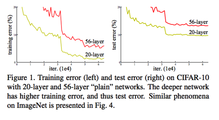
The degradation problem
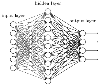
If overfitting is not the reason for degradation, then what is wrong? To explain that, consider the shallow network given below.
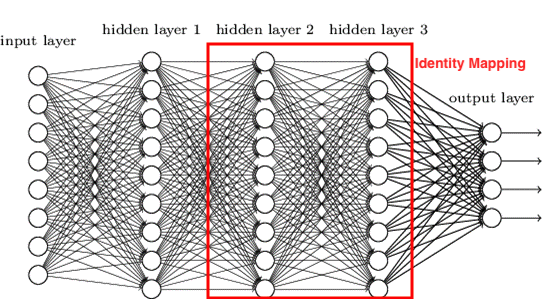
Now let’s make it’s deeper counterpart by stacking up some layers. To make it a counterpart, the added layers should be identity mappings.
Identity mapping or identity function is nothing but $f(x)\ =\ x$. What goes out is what comes in or say, output is same as input. Intuitively, a shallow network plus identity mappings should give a deeper counterpart that shallow network.
Comparing both, what we should expect when it comes to training error of these two networks?
Intuitively, it should be comparable, right ? Or I would say, deeper network will have less training error :/
Yes, but practically, training error of deeper network is more comparing to it’s shallow network.
What? :/
Yeah :)
This experiment expose the culprit behind degradation problem. The added multiple layers fail to learn identity mappings. We thought, if Neural Networks can understand complex patterns, it would be easy for them to understand identity mappings patterns as well. But in this messy real world, Neural Networks train in midst of zombies like vanishing gradients and numerical instability, theories fail. Tough life.
So, how this degradation problem can be solved using ResNets? First let’s see what residual means?
Residual
Residue has a meaning in different fields of math especially in complex analysis. Don’t confuse it with Residual in numerical analysis, which is our area of interest.
Consider the function, \(f(x)\ =\ x^2\)
What is $f(2)$ ? It’s 4.
What about $f(1.99)$ ? It is 3.9601.
So let’s put it this way. I wanted to calculate $f(2)$ but I could compute only an approximation which is $f(1.99)$. So what is the error in computation here?
The error in $x$ is $0.01$.
It is difference in $f(x)$ is $4\ -\ 3.9601\ =\ 0.0399$
This difference is called residual.
A Residual Block
Let’s bring this concept to Neural Nets. Say, two consecutive layers in our network have to learn the mapping $H$. This is the original mapping which is to be learned. It can be identity or complex relationships, we don’t know.
So, if input is $x$, then output after $n$ layers will be $H(x)$. Simple.
Now, we’re going to bring in the residual concept in here. Consider the figure from original paper.
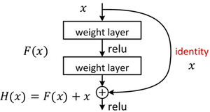
There is a shortcut, hard wired connection from input to output, which is the input $x$ itself. The mapping learned by the layers is not $H(x)$ anymore. It is $F(x)$.
\[F(x)\ =\ H(x)\ -\ x\]Once the shortcut and main path are joined, we get our original mapping $H(x)$. Now, say, when the network needs to learn an identity mapping $H(x)\ =\ x$, it actually learns something else which is not identity.
\[F(x)\ =\ H(x)\ -\ x\ =\ x\ -\ x\ =\ 0\]Since addition with the input will be resultant, though network couldn’t learn anything, the output of a residual block will be,
\[H(x)\ =\ F(x)\ +\ x\ =\ 0\ +\ x\ =\ x\]Woo-Hoo !!! We got the identity mapping ;)
Hypothesis
Residual block is built on the hypothesis that, If one hypothesizes that multiple nonlinear layers can asymptotically approximate complicated functions, then it is equivalent to hypothesize that they can asymptotically approximate the residual functions. Now you ask me how exactly we can prove this hypothesis, I would say it is an open question. People do have different opinions about it. If you would like to read about asymptotic approximation at here. Well, I’m sorry it’s dry. No wait, why should I be sorry? No sorry.
So, here the point is later approach is more easy to learn and it is empirically proved by the authors. I’m going to bring in some equations here, which is already explained in a lite mode.
If $x$ being the input to residual block and $H(x)$ is the original mapping, then,
\[H(x)\ =\ F(x,\ \{W_{i}\})\ +\ x\]Where, $F(x)$ is the relationship learned by the layers, which will be a function with variables input $x$ and weights of the layers embedded in that block. Say for the above block, two layers have respective weights $W_{1}$ and $W_{2}$ and $\sigma$ is the ReLU activation, then,
\[F(x)\ =\ W_{2}*\sigma(W_{1}*x)\]Advantages of Residual Block architecture
- There is no additional parameters to be learned from that shortcut connection since it’s a hard wired input or identity mapping.
- There is no need to alter the learning algorithm, say backpropagation, since our shortcut connection doesn’t disturb the learning procedure anyway. Learning only happens in main path.
- These residuals units can be stacked on one another to bring up a real-deep network without any hassle keeping the above two leverages alive. In the figure given below, left one is our normal,
plainnetwork and the right one is Residual Network (ResNet). Notice the skip connections. With the help of these skip connections, we can train extremely deep networks which will exploit the power of depth which can capture complex patterns in data.
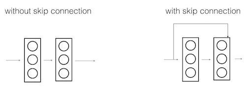
- Skip connections help the input from dying out since the it is hard wired to next layers. This helps to suppress effect of vanishing gradients to a remarkable extent comparing to other techniques.
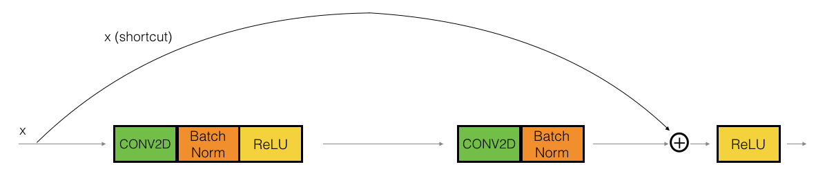
Following figure is another example of residual block with convolution, batch normalization and activations.
The convolutional block
So far discussed about the identity residual block. There is one more type of residual block that are used in a ResNet, depending mainly on whether the input/output dimensions are same or different. What does that mean?
Say we are building a block from 2nd layer to 5th layer and sums up at output of 5th layer. Summing up requires equal dimension vectors, number of activations from 2nd layer and 5th layer should be the same. If is not, then we need to do an additional step in the shortcut connection which can settle this dimension issues. That type of residual block is Convolutional block.
The CONV2D layer in the shortcut path is used to resize the input $x$ to a different dimension, so that the dimensions match up in the final addition needed to add the shortcut value back to the main path.
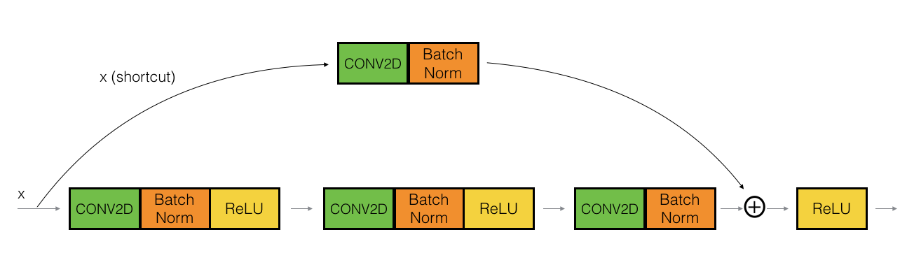
For example, to reduce the activation dimensions’s height and width by a factor of 2, you can use a 1x1 convolution with a stride of 2. The CONV2D layer on the shortcut path does not use any non-linear activation function. Its main role is to just apply a (learned) linear function that reduces the dimension of the input, so that the dimensions match up for the later addition step.
Then our equations will change a bit,
\[H(x)\ =\ F(x,\ \{W_{i}\})\ +\ W_{s}x\]Where $W_{s}$ is called a linear projection.
Linear Projection. What a nice piece of jargon :D
True :D
A linear projection is soley used matching dimensions, since it is empirically proved that, identity mapping is sufficient to solve degradation problem.
Stacking these blocks can help us build Residual Networks. Authors have proposed various models based on them. In the programming session, we’ll build and train a ResNet model named ResNet50, where 50 means 50 layers.
So, that’s it. We’ve learned ResNets neatly. In programming session we’ll convert knowledge to code. See you there :)
I strongly recommend you to read the paper once you complete the tutorial. The authors explain their experiment setups on various datasets and competitions. I would like you to read about Highway Networks too, since Residual Networks has inspiration from that work provided Highway Networks which has many drawbacks when compared to ResNets.
If you think you would like to explore more, this link can provide you the current research innovations on Resnets.
See you in programming session Happy learning :)

Sleeba Paul
Dreamer | Learner | Storyteller